Example Workflows

User Interface: Not applicable.

Scripting: We define a two-dimensional array, analysis_specs, where each row corresponds with one of the three raw heatmaps allQI, allQESV, and allPhi2. Each row contains (1) some text in quotes to use for labelling results, (2) the variable name refering to the raw heatmap in question, and (3) the type of normalization to use for comparing experiment group results to control groups. Here we refer to the normalization types StraightDifference and LogFoldChange. Other available normalization types can be found in the "Normalization Options" dialog.

analysis_specs = [ 
	[ "QI", allQI, StraightDifference ], 
	[ "QESV", allQESV, StraightDifference ], 
	[ "Phi2", allPhi2, LogFoldChange ] 
]

User Interface: Not applicable.

Scripting: We use a pair of square brackets [] to create an empty list, final_results which will be populated later. Then, as in the computation example, we use a for loop to iterate through each row in the analysis_specs defined above. Within the loop, the variable i refers to the current row-index within analysis_specs. For convenience in each loop iteration, we use i to extract three more specific variables from analysis_specs. So, for each loop iteration, paramName, normalizationType, and phi2_raw will be given different values. (Note that wtihin the loop we will always refer to the raw heatmap as phi2_raw regardless of the actual parameter in question.)

final_results = []
for( var i = 0 ; i < analysis_specs.length ; i++ ){
	paramName = analysis_specs[i][0]
	normalizationType = analysis_specs[i][2]
	phi2_raw = analysis_specs[i][1]

User Interface: Follow the "User Interface" steps listed in the normalization example, for each heatmap.

Scripting: Replicate the script from the normalization example, referencing the normalizationType variable in normalization, and paramName in setting titles, and appending normalized results to final_results. (See the full sript at the bottom of this page).

User Interface:

1. Close all heatmaps except for the final results that should be included in the combined visualization
2. At the top of the screen, click "Tools", "Significance Analysis"
3. Click "Launch/Update"
4. Tweek settings and click "Launch/Update" again to update the combined visualization

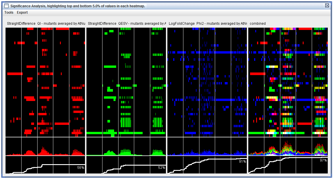
"Significance Analysis" visualization including three component heatmaps where only "significant" cells have been colored, and one combined heatmap (right). Below each heatmap is a gravity plot and cumulative plot giving general views of significance-over-time. Each of the four columns in this visualization can be right-clicked to generate a stand-alone heatmap/spreadsheet.

Scripting: Create a new SignificanceAnalysis object, referencing the final_results list. Then use its getAnalysisResult_PercentileThreshold function. In this example, we use the folowing parameters:

1. Absolute both high and low extremes for each result heatmap should be highlighted. (e.g. both positive and negative extremes).
2. Entire_Map for each result heatmap, each cell value will be compared to the distribution in the entire heatmap to determine whether it should be highlighted.
3. Distinct_Colors Colors for combined result plots will be shown together without blending.
4. false Cumulative plots will NOT be stretched vertically to fill space - this way their vertical axis will be alligned.
5. true Cumultaive plots will be shown separately from gravtiy plots. Otherwise they are superimposed.
6. 5.0 Points are considered significant if they are in the top or bottom fifth percentiel within their heatmap.
7. 1 A single significant timepoints will be considered a "hit" for cumulative-over-time plots. Higher numbers would require significance at multiple adjacent timepoints for cumulative "hits".

sigAnalysis = new SignificanceAnalysis( final_results )
saResults = sigAnalysis.getAnalysisResult_PercentileThreshold( Absolute, Entire_Map, Distinct_Colors, false, true, 5.0, 1)
GLOBAL.display( saResults )

click here to download the full script.

click here to download the sample dataset. This file can be dragged directly into the OLIVER window.

//1 define the type of normalization to use for each heatmap
analysis_specs = [ 
	[ "QI", allQI, StraightDifference ], 
	[ "QESV", allQESV, StraightDifference ], 
	[ "Phi2", allPhi2, LogFoldChange ] 
]

//2 create and empty array to contain results, and begin looping though our analysis_specs
final_results = []
for( var i = 0 ; i < analysis_specs.length ; i++ ){
	paramName = analysis_specs[i][0]
	normalizationType = analysis_specs[i][2]
	phi2_raw = analysis_specs[i][1]
	
    //3 for each iteration of the loop, apply the normalization process
    
	//this is how you would load raw data from harddrive
	//rawDataPath = rawDataFolder + "\\multi-all" + paramName + "_FILTERED_completed_LJS.txt"
	//phi2_raw = GLOBAL.loadHeatMapFromPath(rawDataPath)

	//normalize the experimetn groups against the control groups
    refTable = new ReferenceTable( phi2_raw, "Flat" )
	phi2_lfc = new HeatmapNormalizer( phi2_raw ).buildNormalizedMap( normalizationType, refTable )

	//replace infinite values with blanks
	phi2_lfc.replaceInfiniteValues( NaN )

	//separate control and experiment groups into different heatmaps
	sel_wt = phi2_lfc.searchRowLabels( "col-0" )
	phi2_lfc_wt = phi2_lfc.getSubMap( sel_wt )
	phi2_lfc_mt = phi2_lfc.getSubMap( phi2_lfc.invert( sel_wt ) )

	//create control and experiemnt heatmaps averaged by plantName/Flat
	phi2_lfc_mt_avg = new HeatmapAverager( phi2_lfc_mt ).getAveragedMap( "PlantName", "flat" )
	phi2_lfc_wt_avg = new HeatmapAverager( phi2_lfc_wt ).getAveragedMap( "PlantName", "flat" )

	//create another heatmap averaged by AtNumber
	phi2_lfc_mt_avg_atg = new HeatmapAverager( phi2_lfc_mt_avg ).getAveragedMap( "AtNumber" )

	//reaplcea blanks with zeroes
	phi2_lfc_mt_avg.replaceValues( function(x){ return x=NaN; }, 0 )
	phi2_lfc_wt_avg.replaceValues( function(x){ return x=NaN; }, 0 )
	phi2_lfc_mt_avg_atg.replaceValues( function(x){ return x=NaN; }, 0 )

	//delete non-relevant rows
	phi2_lfc_mt_avg.deleteRows( phi2_lfc_mt_avg.searchRowLabels( "null" ) )
	phi2_lfc_wt_avg.deleteRows( phi2_lfc_wt_avg.searchRowLabels( "null" ) )
	phi2_lfc_mt_avg_atg.deleteRows( phi2_lfc_mt_avg_atg.searchRowLabels( "null" ) )

	//display results in UI
	phi2_lfc_mt_avg.setTitle( normalizationType + " " + paramName + " - mutants averaged by PlantName/Flat" )
	phi2_lfc_wt_avg.setTitle( normalizationType + " " + paramName + " - wildtypes averaged by PlantName/Flat" )
	phi2_lfc_mt_avg_atg.setTitle( normalizationType + "  " + paramName + " - mutants averaged by AtNumber" )
	GLOBAL.display( phi2_lfc_mt_avg, phi2_lfc_wt_avg, phi2_lfc_mt_avg_atg )

	//save the atnumber result for the significance analysis (outside of this loop)
	final_results[i] = phi2_lfc_mt_avg_atg
}

//4 create and display a combined figure using significance analysis
sigAnalysis = new SignificanceAnalysis( final_results )
saResults = sigAnalysis.getAnalysisResult_PercentileThreshold( Absolute, Entire_Map, Distinct_Colors, false, true, 5.0, 1)
GLOBAL.display( saResults )